How To Get A Checkmark In Excel

A check mark is the universal character for confirmed tasks and is widely used in managing lists. Seeing how commonly it's used in organizing ourselves, you would think that there should be a keystroke for this! In this article, we listed 5 methods you can use to to insert a check mark in Excel.

5 Methods to Add a Check Mark in Excel

Copy & Paste

Let's start with the easiest method of adding a check mark in Excel. Copy & Paste the character below:

✓

Enjoy!

Symbols

Excel (as well as Word) has a Symbol feature where all supported characters are listed. You can find the Symbol dialog from the INSERT > Symbols > Symbol path in the Ribbon.

In the Symbol dialog, choose Wingdings from the Font option, and scroll down to find the check mark character. Select the check mark and click the Insert button.

How-to-insert-a-check-mark-in-Excel

Alternatively, you can also type in 252 into the Character code box after selecting the Wingdings font. Knowing the symbol codes can expedite this process quite a bit.

Alt Code

You can enter any special character by typing in the corresponding code. All you need to do is to hold the Alt button, and type in the code. Since the check mark is a symbol that doesn't exist in all font families, you need to set up the required font first.

Set a cell's font type to Wingdings, and while holding the Alt key, press 0252 (the same code from the previous method) in the Symbol dialog.

CHAR Function

The CHAR function simply converts numeric codes into the equivalent ANSI character. For example, the =CHAR(252) formula returns the equivalent character (a check mark) for selected font type. The Wingdings font type should be selected for the check mark to be recognized.

Conditional Formatting

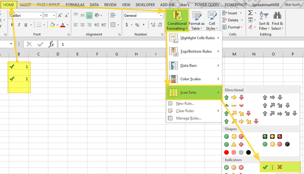
The Conditional Formatting feature can add icons into cells based on cell values and you can use this feature to add a check mark in Excel. For example, you can set rules like "if the cell is equal to 1, then put a check mark".

To apply Conditional Formatting follow the steps below:

Select the range you want place check marks.
Go to HOME > Conditional Formatting > Icon Sets and click the set with check mark.

By default, check marks are associated with ones (1) and crosses with zeros (0). The default rule also calculates the percentiles of the selected range and places check marks for the highest 1/3 of values. To update this rule, click the Manage Rules button under the Conditional Formatting menu while the data range is selected. This will bring up the Conditional Formatting Rules Manager. Double-click on the appropriate rule to edit it. Here you can,